
Thermal Expansion
SYLLABUS
Linear expansion and its measurement, Cubical expansion, superficial expansion and its relation with linear expansion, Liquid Expansion: Absolute and apparent, Dulung and Petit method of determining expansivity of liquid
What is This Chapter About?
Railway tracks have small gaps between sections. Bridges have expansion joints built into their structure. Telephone wires hang with deliberate slack. Thermometers work because mercury expands when heated. All of these are everyday manifestations of a single physical phenomenon — thermal expansion: the tendency of matter to change its dimensions in response to a change in temperature.
When a substance is heated, its molecules gain kinetic energy and vibrate more vigorously. This increased vibration pushes neighbouring molecules slightly further apart on average, causing the substance to expand. When cooled, the reverse happens — molecules move closer together and the substance contracts. This chapter quantifies these changes precisely, introducing the coefficients of expansion that engineers and scientists use to account for temperature-induced dimensional changes in all materials.
Chapter 10 of NEB Grade 11 Physics carries 4 teaching hours and covers both solid and liquid expansion thoroughly. It is a practically grounded chapter with direct connections to engineering, construction, and laboratory measurement.
Key Concepts You Will Learn
Linear Expansion
When a solid rod is heated, its length increases. The coefficient of linear expansion ([latex]\alpha[/latex]) of a material is defined as the fractional increase in length per unit rise in temperature:
[latex]\alpha = \frac{\Delta l}{l_0 \Delta T}[/latex]
So the new length after a temperature rise [latex]\Delta T[/latex] is: [latex]l = l_0(1 + \alpha \Delta T)[/latex].
Different materials have very different values of [latex]\alpha[/latex]. Steel expands relatively little ([latex]\alpha \approx 1.2 \times 10^{-5}[/latex] K⁻¹) while aluminium expands about twice as much. This difference matters enormously in engineering — where steel and aluminium components are joined, their different expansion rates must be accounted for to prevent stress fractures.
Superficial (Area) Expansion
When a solid expands, its surface area also increases. The coefficient of superficial expansion ([latex]\beta[/latex]) relates the fractional increase in area to the temperature change: [latex]\beta = \frac{\Delta A}{A_0 \Delta T}[/latex]. The relationship between superficial and linear expansion is: [latex]\beta = 2\alpha[/latex]. This can be understood geometrically — a square of side l has area [latex]l^2[/latex], and when l increases by a fraction [latex]\alpha \Delta T[/latex], the area increases by approximately [latex]2\alpha \Delta T[/latex].
Cubical (Volume) Expansion
Similarly, the volume of a solid increases with temperature. The coefficient of cubical expansion ([latex]\gamma[/latex]) is defined as: [latex]\gamma = \frac{\Delta V}{V_0 \Delta T}[/latex], and the relationship with linear expansion is: [latex]\gamma = 3\alpha[/latex]. The three coefficients are therefore always in the ratio [latex]\alpha : \beta : \gamma = 1 : 2 : 3[/latex] — a relationship worth memorising.
Measurement of Linear Expansion — Pullinger’s Method
The chapter describes Pullinger’s method for experimentally determining the coefficient of linear expansion of a rod. The rod is heated by steam in a jacket and its change in length is measured using a micrometer or dial gauge. The temperature change is measured with a thermometer. Plotting the graph of length against temperature gives a straight line whose gradient is [latex]l_0 \alpha[/latex], allowing [latex]\alpha[/latex] to be calculated precisely.
Force Due to Expansion and Contraction
If a solid is prevented from expanding when heated — as happens with railway tracks constrained between fixed supports — enormous internal stresses build up. The force generated is: [latex]F = YA\alpha\Delta T[/latex], where Y is Young’s modulus. This thermal stress can be sufficient to buckle railway tracks or crack concrete structures if expansion joints are not provided. Conversely, cooling a constrained rod generates tensile stress — this principle is used in shrink fitting, where a metal ring is heated, placed over a shaft, and then cooled to grip it tightly.
Differential Expansion
When two different materials are bonded together and heated, they expand by different amounts. This differential expansion causes the composite system to bend. This is the principle behind the bimetallic strip — two strips of different metals (typically brass and invar) bonded together. When heated, the metal with the higher [latex]\alpha[/latex] expands more, causing the strip to curve toward the metal with lower expansion. Bimetallic strips are used in thermostats, circuit breakers, and mechanical thermometers.
Variation of Density with Temperature
Since volume increases with temperature while mass remains constant, density decreases with increasing temperature: [latex]\rho = \frac{\rho_0}{1 + \gamma \Delta T}[/latex]. This variation of density with temperature drives convection currents — warmer, less dense fluid rises while cooler, denser fluid sinks — which is the mechanism behind sea breezes, atmospheric circulation, and convective heat transfer in oceans and stars.
Expansion of Liquids — Apparent and Real Expansion
Liquids expand more than solids. However, measuring liquid expansion is complicated by the fact that the container itself also expands. What we directly observe is the apparent expansion — the expansion of the liquid relative to the container. The real expansion of the liquid is the sum of the apparent expansion and the expansion of the container:
[latex]\gamma_{real} = \gamma_{apparent} + \gamma_{glass}[/latex]
Or in terms of the coefficients: [latex]\gamma_r = \gamma_a + \gamma_g[/latex]. This distinction is crucial for accurate thermometry and volumetric measurements.
Dulong and Petit’s Experiment
Dulong and Petit’s method determines the absolute (real) expansivity of a liquid by comparing its density at two different temperatures using a U-tube manometer. Since the pressure at the bottom of both arms of the U-tube must be equal, the heights of liquid columns at different temperatures give the ratio of densities, from which the real cubic expansivity can be calculated without needing to know the expansion of the container separately.
Why This Chapter Matters for NEB Exams
Thermal Expansion is examined consistently in NEB Grade 11 Physics. The relationship [latex]\gamma = 3\alpha[/latex] and [latex]\beta = 2\alpha[/latex], the distinction between apparent and real expansion of liquids, and the principle of Pullinger’s method are standard examination questions. Numerical problems involving linear expansion, calculation of new dimensions, and thermal stress in constrained rods appear regularly. Differential expansion and bimetallic strips are popular application-based questions. The formula for real expansion of liquids is a frequent short-answer topic.
Important Topics to Focus On
- Coefficient of linear expansion [latex]\alpha[/latex] — definition and formula
- Superficial expansion [latex]\beta[/latex] and cubical expansion [latex]\gamma[/latex] — definitions and relation [latex]\gamma = 3\alpha[/latex], [latex]\beta = 2\alpha[/latex]
- Pullinger’s method for determining [latex]\alpha[/latex]
- Thermal stress in constrained rods: [latex]F = YA\alpha\Delta T[/latex]
- Differential expansion and bimetallic strips — applications
- Variation of density with temperature
- Real and apparent expansion of liquids: [latex]\gamma_r = \gamma_a + \gamma_g[/latex]
- Dulong and Petit’s experiment — principle and method
- Numerical problems on all expansion topics
Connection to Other Chapters
Thermal Expansion connects backward to Chapter 9 (Heat and Temperature) — temperature change drives expansion — and forward to Chapter 11 (Quantity of Heat), where specific heat capacity determines how much heat is needed to produce that temperature change. The thermal stress formula uses Young’s modulus from Chapter 8 (Elasticity), beautifully connecting the two branches of mechanics and heat. The variation of density with temperature drives convection, which is central to Chapter 12 (Rate of Heat Flow). In Grade 12, thermal expansion of gases is central to the ideal gas law in Chapters 4 and 5 (Thermodynamics).
The increase in size of a body on heating is called thermal expansion.
Expansion of Solids
In solids, molecules are held by strong intermolecular forces between the molecules. So, expansion in solids is small. When it is heated, its atoms vibrate about their mean position and their amplitude increases. So, equilibrium distance between them increases, which increases its size.
1. Linear Expansion
If a substance in the form of rod or wire is heated, its length increases. Such type of expansion is called linear expansion. It does not mean that there is no expansion in area and volume. However, the expansion of area and volume in insignificant as compared to the expansion in length.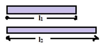
Let a metal rod has length l1 at temperature [latex]\theta_1[/latex]. When it is heated up to the temperature [latex]\theta_2[/latex], its length increases & becomes l2. Thus, the change in length [latex](\Delta l) = l_2-l_1[/latex] & change in temperature [latex](\Delta \theta) = \theta_2 – \theta_1[/latex]. Thus, the change in length [latex](\Delta l)[/latex] is directly proportional to
(i) The original length, i.e.
[latex]\Delta l \propto[/latex] l1
The rise in temperature, i.e.
[latex]\Delta l \propto \Delta \theta = (\theta_2 – \theta_1)[/latex]
Combining both, we get,
[latex]\Delta l \propto l_1 (\theta_2 – \theta_1)[/latex]
[latex]\Delta l = \alpha l_1(\theta_2 – \theta_1)[/latex] ……….. (1)
Where, [latex]\alpha[/latex] is a proportionality constant, called coefficient of linear expansion.
From equation (1), we get,
[latex]\alpha = \frac{\Delta l}{l_1 (\theta_2 – \theta_1)}[/latex] ………………………………….. (2)
= [latex]\frac{change\ in\ length}{original\ length \times change\ in\ temperature}[/latex]
If l1 = 1 unit, [latex]\theta_2 – \theta_1[/latex] = 1 unit, then, [latex]\alpha = \Delta l[/latex].
Thus, the coefficient of linear expansion may be defined as the change in length to the per unit original length per unit change in temperature. Its value is different for different materials.
From eqn. (1), we get,
l2-l1 = [latex]\alpha l_1 \Delta \theta[/latex]
Or, l2 = l1 + l1[latex]\alpha \Delta \theta[/latex]
[latex]l_2 = l_1 (1+\alpha \Delta \theta)[/latex] …………………………… (3)
Unit of [latex]\alpha[/latex]
The unit of [latex]\alpha[/latex] is oC-1 or K-1.
2. Superficial Expansion
The increase in area with rise in temperature is called superficial expansion.
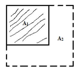
Let us consider, a metal sheet has an area A1 at temperature [latex]\theta_1[/latex]. When it is heated up to [latex]\theta_2[/latex], its area increases & becomes A2. Thus, the change in area, [latex]\Delta A[/latex] = (A2-A1) & change in temperature [latex]\Delta \theta[/latex] = [latex](\theta_2 – \theta_1)[/latex]. Experimentally, the change in area is:
i. Directly proportional to the original area. i.e.
[latex]\Delta A \propto A_1[/latex] ……………….. (1)
ii. Directly proportional to the change in temperature. i.e.
[latex]\Delta A[/latex] ∝ (θ2-θ1). ……………. (2)
Combining both, we get,
[latex]\Delta A \propto A_1(\theta_2 – \theta_1)[/latex]
Or, [latex]\Delta A = \beta A_1(\theta_2 – \theta_1)[/latex] ………………………… (3)
Where, β is the proportionality constant, called coefficient of superficial expansion.
From eqn. (3), we get,
[latex]\beta = \frac{\Delta A}{A_1(\theta_2 – \theta_1)}[/latex]
= [latex]\frac{\text{Change in Area}}{\text{original area}\times \text{change in temperature}}[/latex]
If A1 = 1 unit, [latex]\theta_2 – \theta_1[/latex] = 1 unit, then β = [latex]\Delta A[/latex]
Hence, the coefficient of superficial expansion may be defined as the change in area per unit original area per unit change in temperature.
From eqn. (3), we get,
A2-A1 = β A1 [latex]\Delta \theta[/latex]
Or, A2 = A1 (1+β[latex]\Delta \theta[/latex])
Unit of β
Its unit is oC-1 or K-1.
3. Cubical Expansion:
The expansion in volume with rise in temperature is called cubical expansion.
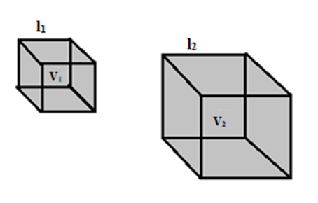
Let us consider, an object has volume [latex]V_1\ at\ θ_1[/latex] temperature. When it is heated upto temperature [latex]θ_2[/latex], its volume increases and becomes [latex]V_2[/latex]. Thus, the change in volume ∆V = [latex](V_2-V_1)[/latex] and change in temperature ∆θ = [latex](θ_2-θ_1)[/latex]. Thus, the change in volume is directly proportional to:
i. The original volume. i.e.
[latex]\Delta V \propto V_1[/latex]
ii. The rise in temperature. i.e.
[latex]\Delta V \propto (\theta_2 – \theta_1)[/latex]
Combining both, we get,
[latex]\Delta V \propto V_1(\theta_2 – \theta_1)[/latex]
[latex]\Delta V = \gamma V_1(\theta_2 – \theta_1) \dots\dots\dots\dots\dots\dots\dots\dots\dots\dots\dots (1)[/latex]
Where, γ is the proportionality constant called coefficient of cubical expansion.
From eqn. (1), we get,
[latex]\gamma = \dfrac{\Delta V}{V_1(\theta_2-\theta_1)} = \dfrac{change\ in\ volume}{original\ volume\ \times change\ in\ temperature}[/latex]
If [latex]V_1[/latex] = 1 unit & [latex](θ_2-θ_1)[/latex] = 1 unit, then, γ = ∆V.
Thus, cubical expansion may be defined as the change in volume per unit original volume per unit change in temperature.
From eqn. (1), we get,
[latex]V_2-V_1 = \gamma V_1 \Delta\theta[/latex]
[latex]V_2 = V_1(1+\gamma\Delta\theta)[/latex]
Unit of γ:
Its unit is [latex]^oC^{-1}\ or\ K^{-1}[/latex]
Relation between coefficients of expansion:
Relation between α and β:
Let us consider, a square plate of side [latex]l_1[/latex] at temperature [latex]θ_1[/latex] & [latex]l_2[/latex] at [latex]θ_2[/latex] as shown in the given figure. Then,
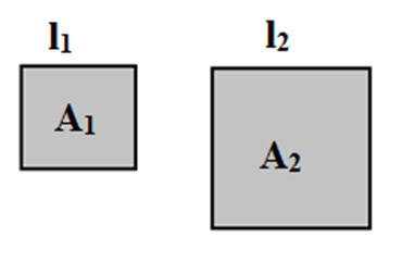
[latex]l_2 = l_1(1+\alpha\Delta\theta)[/latex]
Where, α is the coefficient of linear expansion.
Area of the plate at [latex]θ_1 (A_1) = l_1^2[/latex]
Area of the plate at [latex]θ_2 (A_2) = l_2^2[/latex]
[latex]= l_1^2(1+\alpha\Delta\theta)^2[/latex]
[latex]= A_1(1+\alpha\Delta\theta)^2 \dots\dots (1)[/latex]
Area of the plate at [latex]θ_2[/latex] is also given by:
[latex]A_2 = A_1(1+\beta\Delta\theta) \dots\dots\dots\dots (2)[/latex]
Where, β is the coefficient of superficial expansion.
From eqns. (1) and (2), we get,
[latex]A_1(1+\beta \Delta \theta) = A_1(1+\alpha \Delta \theta)^2[/latex]
Or, [latex](1+\beta \Delta \theta) = 1 + 2\alpha\Delta\theta + \alpha^2\Delta\theta^2[/latex]
Or, [latex]\beta\Delta\theta = 2\alpha\Delta\theta + \alpha^2\Delta\theta^2[/latex]
Since, α is very small, the term containing higher power of α can be neglected. Thus,
[latex]\beta\Delta\theta = 2\alpha\Delta\theta[/latex]
[latex]\beta = 2\alpha \dots\dots\dots\dots\dots\dots (3)[/latex]
Hence, the coefficient of superficial expansion of a solid is twice the value of linear expansion.
Relation between α and γ:
Let us consider, a cubical plate of side [latex]l_1\ at\ θ_1\ \&\ l_2\ at\ θ_2[/latex] as shown in the given figure. Also, let, volume [latex]V_1\ at\ θ_1\ \&\ V_2[/latex] at [latex]θ_2[/latex]. Then,
[latex]l_2 = l_1(1+\alpha\Delta\theta)[/latex]
Where, α is the coefficient of linear expansion.
Volume of the cube at [latex]θ_1 = V_1 = l_1^3[/latex]
Volume of the cube at [latex]θ_2 = V_2 = l_2^3[/latex]
Or, [latex]V_2 = l_1^3(1+\alpha\Delta\theta)^3[/latex]
∴ [latex]V_2 = V_1(1+\alpha\Delta\theta)^3 \dots\dots\dots.\dots (1)[/latex]
Also, the volume of the cube at [latex]θ_2[/latex],
[latex]V_2 = V_1(1+\gamma\Delta\theta) \dots\dots\dots\dots\dots\dots\dots\dots\dots. (2)[/latex]
From eqns. (1) and (2), we get,
[latex]V_1(1+\alpha\Delta\theta)^3 = V_1(1+\gamma\Delta\theta)[/latex]
[latex]1 + 3\alpha\Delta\theta + 3\alpha^2\Delta\theta^2 + \alpha^3\Delta\theta^3 = 1+\gamma\Delta\theta[/latex]
Or, [latex]3\alpha\Delta\theta + 3\alpha^2\Delta\theta^2 + \alpha^3\Delta\theta^3 = \gamma\Delta\theta[/latex]
Since, α is very small, the term containing higher power of α can be neglected. Thus,
[latex]3\alpha\Delta\theta = \gamma\Delta\theta[/latex]
Or, [latex]3\alpha = \gamma[/latex]
Hence, coefficient of cubical expansion of a solid is three times the coefficient of linear expansion.
Relation between α, β and γ:
We have, [latex]\beta = 2\alpha[/latex]
Or, [latex]\alpha = \dfrac{\beta}{2}[/latex]
Also, [latex]\gamma = 3\alpha[/latex]
[latex]\alpha = \dfrac{\gamma}{3}[/latex]
Hence, [latex]\alpha = \dfrac{\beta}{2} = \dfrac{\gamma}{3}[/latex]
[latex]\alpha : \beta : \gamma[/latex] = 1:2:3
Coefficient of Linear Expansion of a solid by Pullinger’s Apparatus
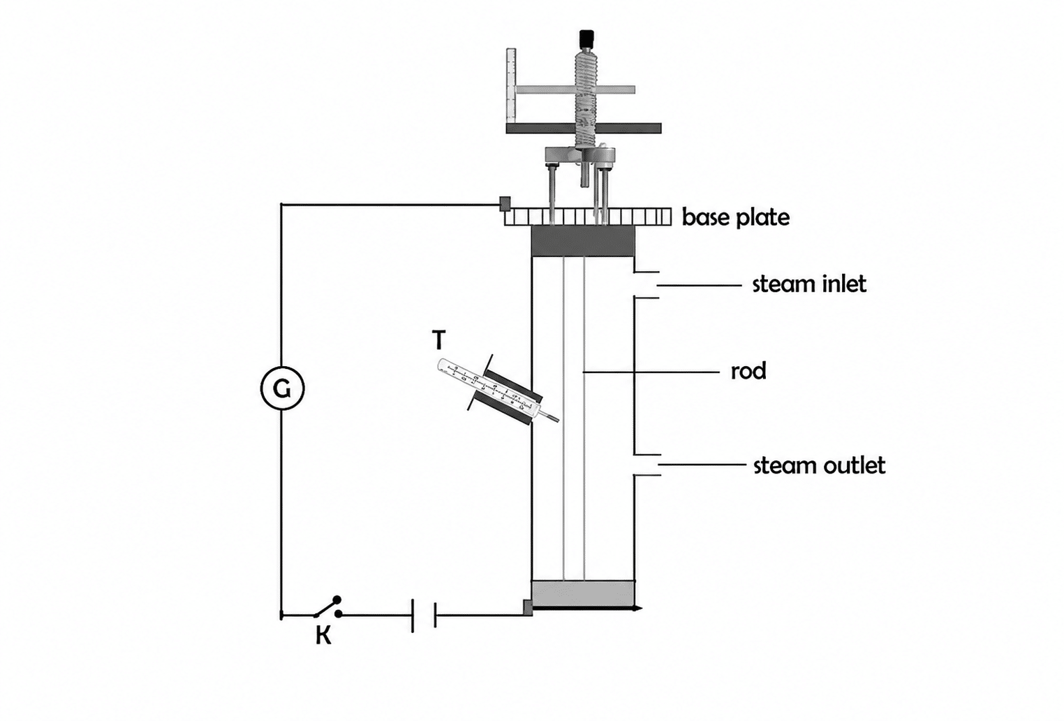
The experimental method to determine coefficient of linear expansion is as shown in figure. It consists of steam chamber having three holes for steam inlet, steam outlet and thermometer. An experimental rod is placed vertically at the middle of steam chamber. From the two ends of the rod, a galvanometer is connected along with the cell as shown in figure. And, spherometer is placed at the top of rod. The galvanometer shows deflection when central leg of spherometer touches the rod. Now, steam is passed from steam inlet and recorded the temperature by thermometer. And the expansion of metal rod is measured by spherometer.
Let,
Initial length of rod = l1
Initial temperature of rod = [latex]\theta_1^oC[/latex]
Final temperature of rod = [latex]\theta_2^oC[/latex]
Initial reading of spherometer = R1
Final reading of spherometer = R2
Now, from the definition of linear expansion
[latex]\alpha = \frac{Change\ in\ length}{Original\ length\ \times\ change\ in\ temperature}[/latex]
[latex]\alpha = \frac{R_2 – R_1}{l_1(\theta_2 – \theta_1)}[/latex]
This is the required expression for coefficient of linear expansivity from Pullinger’s apparatus.
Differential Expansion
Different metals have different coefficient of expansion. The difference in expansion of the bodies when they are heated by the same range of temperature is called differential expansion.
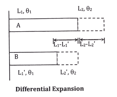
Let us consider, two rods A & B having the lengths L1 & L1‘ respectively at temperature [latex]\theta_1[/latex]. They are heated upto temperature [latex]\theta_2[/latex] such that their length becomes L2 & L2‘ respectively. Then, we have,
At temperature [latex]\theta_1, d_1 = L_1 – L_1^{‘}[/latex] …….. (i)
Similarly, at temperature [latex]\theta_2, d_2 = L_2 – L_2^{‘}[/latex] ………… (ii)
We also have,
L2 = L1 [latex](1+\alpha \Delta \theta)[/latex] ………………… (iii)
And, L2‘= L1‘ [latex](1+\alpha^{‘} \Delta \theta)[/latex] ……………….. (iv) Where, α and α‘ are the coefficients of linear expansivities of A and B.
Now, From eqn. (ii),
d2 = L2 – L2‘
= [latex]L_1(1+\alpha \Delta \theta) – L_1^{‘}(1+\alpha^{‘} \Delta \theta)[/latex]
= L1 + L1 α[latex]\Delta \theta[/latex] – L1‘ – L1‘ α‘[latex]\Delta \theta[/latex]
= (L1 – L1‘) + (L1α – L1‘ α‘)[latex]\Delta \theta[/latex]
= d1 + (L1α – L1‘ α‘)[latex]\Delta \theta[/latex]
[latex]\therefore[/latex] d2 – d1 = (L1α – L1‘ α‘)[latex]\Delta \theta[/latex]
This is an expression for differential expansion.
If the original lengths & materials of the bodies are so chosen that, they always have the same expansion, then,
[latex]d_2 – d_1 = 0[/latex]
(L1α – L1‘ α‘)[latex]\Delta \theta[/latex] = 0
Then, [latex]\frac{L_1}{L_1^{‘}} = \frac{\alpha^{‘}}{\alpha}[/latex]
i.e., if the lengths of the rods are inversely proportional to their linear expansivity, then, the difference between the lengths is constant at all temperature.
Force or Stress set up in rod due to expansion or contraction:
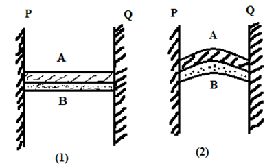
Consider, a rod R of length [latex]l_1[/latex] fixed between two rigid supports P & Q at temperature [latex]θ_1[/latex]. When the rod is heated upto [latex]θ_2[/latex], it expands and its length increases & becomes [latex]l_2[/latex]. Due to increase in temperature, the rod tries to expand but will not be able to expand due to rigid ends, as a result, a force or tension is produced, which would compress the rod.
The corresponding length [latex](l_2)[/latex] is given by:
[latex]l_2 = l_1(1+\alpha\Delta\theta)[/latex]
Where, α = Coeff. Of linear expansion of material of rod.
Or, [latex]l_2 – l_1 = l_1\alpha\Delta\theta[/latex]
∴ Increase in length (e) = [latex]l_1\alpha\Delta\theta[/latex] ……………………….. (1)
If Y be the Young’s modulus of elasticity of the material of rod, then,
[latex]Y = \dfrac{Stress}{Strain}[/latex]
Stress: The ratio of force to the area is called stress.
Strain: The ratio of increase in length to the original length is called strain. i.e.
[latex]Stress = \dfrac{Force\ (F)}{Area\ (A)} = \dfrac{F}{A} = \dfrac{Tension}{Area}[/latex]
[latex]Strain = \dfrac{Increase\ in\ length\ (e)}{Original\ length\ (l_1)} = \dfrac{e}{l_1}[/latex]
[latex]= \dfrac{l_1\alpha\Delta\theta}{l_1}[/latex] [∵ From eqn. (1)]
[latex]= \alpha\Delta\theta[/latex]
Young’s Modulus (Y) = [latex]\dfrac{Stress}{Strain}[/latex]
∴ [latex]Y = \dfrac{F/A}{\alpha\Delta\theta}[/latex]
[latex]\dfrac{F}{A} = Y\alpha\Delta\theta[/latex]
∴ [latex]F = YA\alpha\Delta\theta[/latex]
Expansion of Liquid
Liquids, just like solids expands on heating & contracts on cooling. The expansion on liquid is more than that of the solid. It is because, the intermolecular force of attraction on liquid is less than that of solid. So, the molecules vibrate quickly on liquid than solid.
For the study of expansion of liquid, we have to study about the cubical expansion. We know, liquid have no shape but have definite volume. When it is kept in a vessel & then heated, the volume of liquid as well as the vessel increases.
Real & Apparent expansion of a liquid
The expansion of liquid on rise in temperature is always associated with the expansion of vessel. The expansion, which we observe is called apparent expansion. It is always less than real expansion of the liquid.
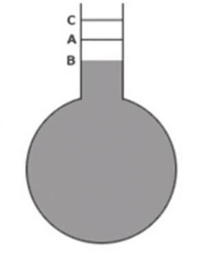
Let us take a round bottom flask made of glass with long narrow stem. Let, it be filled with liquid upto A. If the bulb is immersed in a hot liquid bath, the liquid level comes down to B. This is because the vessel is heated before the liquid. So, it expands first and the level of liquid decreases. After this, the liquid is heated and its level rises to C.
So, real expansion of liquid = increase in volume from B to C
Or, real expansion of liquid = increase in volume from B to A + increase in volume from A to C
Or, real expansion of liquid = expansion of vessel + apparent expansion of liquid
i.e., VBC = VAB + VAC ………………… (i)
Relation between Coefficient of Real and Apparent Expansion
Let us consider, a liquid contained in a vessel at room temperature [latex]\theta_1[/latex]. If V be the original volume, then, suppose, the liquid is heated to temperature [latex]\theta_2[/latex]. So,
Coefficient of real expansion of liquid [latex](\gamma_r) = \frac{Real\ increase\ in\ volume}{Original\ volume \times rise\ in\ temperature}[/latex]
= [latex]\frac{V_{BC}}{V\times \Delta \theta}[/latex]
[latex]V_{BC} = V\gamma_r \Delta \theta[/latex]
Also, coefficient of apparent expansion of liquid [latex](\gamma_a)[/latex]
= [latex]\frac{\text{Apparent increase in volume}}{Original\ volume \times rise\ in\ temperature}[/latex]
= [latex]\frac{V_{AC}}{V\times \Delta \theta}[/latex]
Or, VAC = [latex]V\gamma_a \Delta \theta[/latex]
Now, coefficient of volume expansion of glass vessel [latex](\gamma_g)[/latex]
= [latex]\frac{\text{Increase in volume of vessel}}{Original\ volume \times rise\ in\ temperature}[/latex]
= [latex]\frac{V_{AB}}{V\times \Delta \theta}[/latex]
Or, VAB = [latex]V\gamma_g \Delta \theta[/latex]
So, from equation (i),
VBC = VAB + VAC
Or, [latex]V\gamma_r \Delta = V\gamma_g \Delta \theta + V\gamma_a \Delta \theta[/latex]
Or, [latex]\gamma_r = \gamma_g + \gamma_a[/latex]
This is the required relation between coefficients of real and apparent expansivity of a liquid.
Determination of the co-efficient of real expansion of a liquid by Dulong and Petit’s method
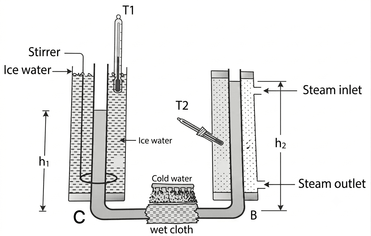
The apparatus consists of a U- shaped tube which contains liquid whose coefficient of real expansion is to be determined. The vertical limbs are surrounded by glass jackets. One jacket is placed with ice water and another jacket is placed at steam temperature by passing steam continuously through it. The horizontal part of the tube is continuously cooled by spraying cold water on it to prevent the flow of heat due to conduction across it. Ice water and steam is passed for a long time until it attains steady state separately and the temperatures are noted.
Calculation
Let, the temperatures of the cold and hot limbs be [latex]\theta_1^oC[/latex] and [latex]\theta_2^oC[/latex] respectively. For the liquid to be in steady state, the pressure at B must be equal to the pressure at C.
If h1 and h2 be the heights of the liquid columbs and [latex]\rho_1[/latex] and [latex]\rho_2[/latex] be the densities of the liquid at temperatures [latex]\theta_1^oC[/latex] and [latex]\theta_2^oC[/latex] respectively, then,
[latex]h_1\rho_1 g = h_2\rho_2 g[/latex] ………………….. (i)
[latex]\frac{h_1}{h_2} = \frac{\rho_2}{\rho_1}[/latex] ……………….. (ii)
But, density at [latex]\theta_2[/latex],
[latex]\rho_2 = \frac{\rho_1}{1+\gamma \Delta \theta}[/latex] ………………….. (iii)
And from eqn. (ii), we get,
[latex]\frac{h_1}{h_2} = \frac{\rho_1}{\rho_1(1+\gamma \Delta \theta)}[/latex]
Or, [latex]h_2 = h_1 + h_1 \gamma \Delta \theta[/latex]
[latex]\therefore h_2 – h_1 = h_1 \gamma \Delta \theta[/latex]
Or, [latex]\gamma = \frac{h_2 – h_1}{h_1\Delta \theta}[/latex]
By knowing the values of RHS, the coefficient of real expansion of liquid can be determined.
MCQs
A piece of copper wire has a length of 100 cm at 5oC. Its length at 478 K will be (given: [latex]\alpha = 17\times 10^{-6}[/latex] oC-1)
Show answer
Which of the following is correct for solids?
Show answer
The increase in length of a body of 50 meter length is 2.3 mm when the body is heated from 0oC to 50oC. The coefficient of linear expansion of the body is
Show answer
Lengths of two metal bars ‘A’ and ‘B’ are 8 cm and 12 cm respectively. If they show same difference in lengths at all temperature, their superficial expansivities are in the ratio
Show answer
A clock has copper pendulum beats seconds correctly when temperature of the room is 30oC, the time loss or gain per day when temperature falls to 10oC is ([latex]\alpha = 1.9\times 10^{-5} K^{-1}[/latex]).
Show answer
Which material has least value of expansivity?
Show answer
The ratio of real expansivity to apparent expansivity of a liquid is
Show answer
Theoretical questions
Two metallic rods of the same material but of different length are heated. Smaller rod has circular area of cross – section but larger rod had rectangular cross – section. Will their linear expansivity be the same or different? Give justification of your answer.
Why is it sometimes possible to loosen caps on screw top bottles by dipping the cap briefly in hot water?
Explain why the possibility of “water taps burst” rise in severe winter.
A square brass plate has a large circular hole cut in its centre. If the plate is heated, it will expand. Will the diameter of the hole expand or contract? Explain your answer.
Define the coefficient of cubical expansion of a solid and hence write an expression for the variation of its density with temperature.
Frozen water pipes often burst. Will an alcohol thermometer break if the temperature drops below the freezing point of alcohol?
A hole is drilled in a flat metal sheet. What happens to the diameter of the hole as the metal sheet is heated to higher temperature?
Does the cubical expansivity of a liquid depend on its original volume? Explain.
Frozen water pipes often burst; will a mercury thermometer break if the temperature of the thermometer is brought below the freezing point of mercury?
Does the coefficient of linear expansion depend on length? Justify your answer.
Why are glass windows possible to be cracked in very cold region?
Two bodies made of the same material have the same external dimension and appearance, but one is solid and the other is hollow. When they are heated, is the overall volume expansion the same or different?
Why does a thick glass tumbler crack when boiling water is poured on it?
Water level initially falls in a vessel when it is heated. Why?
Define coefficients of real and apparent expansion of a liquid and establish a relation between them.
Define the coefficients of linear and cubical expansion of solid and establish their relation.
Describe how the cubical expansivity of a liquid can be determined by the use of balanced columns.
Distinguish between real and apparent expansion of liquid. Describe with mathematical detail, a method to determine real expansivity of a liquid.
Describe a method to determine the linear expansivity of a solid. Can the cubical expansivity be derived from this value?
Define linear and cubical expansivities of solids. Derive an expression for the variation in density of a solid when its temperature is raised from [latex]\theta_1^oC[/latex] to [latex]\theta_2^oC[/latex].
Define linear, superficial and cubical expansivities. Show that [latex]\beta = 2\alpha[/latex] where [latex]\alpha[/latex] and [latex]\beta[/latex] are linear and superficial expansivities.
Why do substances expand on heating? Show that [latex]\alpha = \frac{\gamma}{3}[/latex], where [latex]\alpha[/latex] and [latex]\gamma[/latex] are the coefficients of linear and cubical expansions of a substance.
Obtain an expression for the change in density of a gas due to the thermal expansion.
Numerical problems
A glass flask of volume 400 cm3 is just filled with mercury at 0oC. How much mercury overflows when the temperature of the system is raised to 80oC? The coefficient of cubical expansivity of glass is 1.2 x 10⁻⁵ oC-1 and that of mercury is 1.8 x 10⁻⁵ oC-1. Ans: [latex]0.192\ cm^3[/latex]
A glass flask with volume 200 cm3 is filled to the brim with mercury at 20oC. How much mercury overflows when the temperature of the system is raised to 100oC? (Linear expansivity of glass = 0.4 x 10⁻⁵ K-1, cubical expansivity of mercury = 18 x 10-5 K-1). Ans: 2.688 cm3
A glass vessel of volume 50 cm3 is filled with mercury and is heated from 20oC to 60oC. What volume of mercury will overflow? Cubical expansivity of glass = 1.8 x 10⁻⁶ K-1 and cubical expansivity of mercury = 1.8 x 10⁻⁴ K-1. Ans: 0.3564 cm3
A glass flask of volume 500 cm3 is just filled with mercury at 0oC. how much mercury overflows when the temperature of the system is raised to 80oC? Ans: 0.24 cm3
A copper vessel with a volume of exactly 100 m3 at a temperature of 15oC is filled with glycerine. If the temperature rises to 25oC, how much glycerine will spill out? Ans: 0.48 m3
An iron rod of length 100 m at 10oC is used to measure a distance of 2 km on a day when the temperature is 40oC. Calculate the error in measuring the distance. [latex](\alpha[/latex] for iron = 12 x 10-6 oC-1). Ans: 72 cm
The marking on an aluminium ruler and a brass ruler are perfectly aligned at 0oC. How far apart will the 20.0 cm marks be on the two rulers at 100oC, if precise alignment of the left-hand ends of the rulers is maintained? Coefficient of linear expansion of aluminium and brass are 2.4 x 10⁻⁵ K-1 and 2.0 x 10⁻⁵ K-1 respectively. Ans: 0.008 cm
The length of an iron rod is measured by a brass scale. When both of them are at 10oC, the measured length is 50 cm. What is the length of the rod of 40oC when measured by the brass scale at 40oC? [latex](\alpha[/latex] for brass = 24 x 10-6 oC-1,[latex]\alpha[/latex] for iron = 16 x 10-6 oC-1). Ans: 49.98 cm
A second pendulum made of brass keeps correct time at 10oC. How many seconds it will lose or gain per day when the temperature of its surrounding rises to 35oC? [latex](\alpha[/latex] for brass =[latex]2\times 10^{-5}[/latex] oC-1). (2074 ‘A’)Ans: 21.168 s lose per day
A brass pendulum clock keeps correct time at 15oC. How many seconds per day it will lose or gain at 0oC? [latex](\alpha [/latex] for brass = [latex]2\times 10^{-5}K^{-1})[/latex] Ans: 12.96 s gain
An iron pendulum clock keeps correct time at 20oC. How many seconds will it gain or lose per day when temperature rises to 30oC? (2069 ‘S’)Ans: 5.18 s per day
The pendulum of a clock is made of brass. If the clock keeps correct time at 15oC, how many seconds per day will it lose at 20oC? Ans: 4 s
A pendulum clock made of iron keeps correct time at 15oC. How many seconds will it lose or gain per day when the temperature rises to 35oC? Ans: 20.7 s
A clock which has a brass pendulum beats seconds correctly when the temperature of the room is 30oC. How many seconds will it gain or lose per day when the temperature of the room falls to 10oC? [latex](\alpha[/latex] for brass = 0.000018 oC-1). Ans: 16.92 s gain
A steel wire 8m long and 4 mm in diameter is fixed to two rigid supports. Calculate the increase in tension when the temperature falls by 10oC. (Young’s modulus of elasticity of steel = 2 x 10¹¹ N/m2 and linear expansivity of steel = 1.2 x 10⁻⁵ K-1). Ans: 302.4 N
A copper wire of diameter 0.5 mm is stretched between two points at 25oC. Calculate the increase in tension in the wire if the temperature falls to 0oC. (Young’s modulus for copper = 1.2 x 10¹¹ Nm-2), linear expansivity for copper = 18 x 10-6 K-1). Ans: 10.6 N
The density of silver at 0oC is 10310 kgm-3 and the coefficient of linear expansion is 0.000019/oC. Calculate its density at 100oC. Ans: 10251.57 kg/m3
Using the following data, determine the temperature at which wood will just sink in benzene. Density of benzene at 0oC = 9.0 x 10² Kgm-3, Density of wood at 0oC = 8.8 x 10² Kgm-3. (Cubical expansivity of benzene = 1.2 x 10⁻³ K-1, Cubical expansivity of wood = 1.5 x 10⁻⁴ K-1). Ans: 21.07oC
A brass rod of length 0.40 m and steel rod of length 0.60 m, both are initially at 0oC are heated to 75oC. If the increase in length is the same for both the rods, calculate the linear expansivity of brass. The linear expansivity of steel is 12 x 10-6 oC-1. Ans: 18 x 10-6 oC-1
A glass flask of volume 400 cm3 is just filled with mercury at 0oC. How much mercury overflows when the temperature of the system is raised to 80oC? The coefficient of cubical expansivity of glass is 1.2 x 10⁻⁵ oC-1 and that of mercury is 1.8 x 10⁻⁵ oC-1.
Solution
For glass flask,
Volume (V1) = 400 cm3
Initial temperature [latex](\theta_1)[/latex] = 0oC
Final temperature [latex](\theta_2)[/latex] = 80oC
Change in temperature [latex](\Delta \theta) = \theta_2 – \theta_1[/latex] = 80 – 0 = 80oC
Coefficient of cubical expansivity of glass [latex](\gamma_g)[/latex] = 1.2 x 10⁻⁵ oC-1
Volume of glass flask at 80oC (V2) = [latex]V_1(1+\gamma_g \Delta \theta)[/latex]
= 400(1+ 1.2 x 10-5 x 80)
= 400.38 cm3
Now, for mercury,
Volume (V1) = 400 cm3 [∵ glass flask is just filled with mercury]
Coefficient of cubical expansivity of mercury [latex](\gamma_{Hg})[/latex] = 1.8 x 10⁻⁵ oC-1
Volume of mercury at 80oC (V2‘) = [latex]V_1(1+\gamma_{Hg}\Delta \theta)[/latex]
= 400(1+ 1.8 x 10-5 x 80)
= 400.58 cm3
So, Volume of mercury overflows = V2‘ – V2
= 400.58 – 400.38
= 0.2 cm3
= 2 x 10⁻⁷ m3
A glass flask with volume [latex]200\ cm^3[/latex] is filled to the brim with mercury at 20°C. How much mercury overflows when the temperature of the system is raised to 100°C? (Linear expansivity of glass = [latex]0.4\times10^{-5}\ K^{-1}[/latex], cubical expansivity of mercury = [latex]18\times10^{-5}\ K^{-1}[/latex]).
Solution
For glass flask,
Volume [latex](V_1) = 200\ cm^3[/latex]
Initial temperature [latex](\theta_1) = 20^oC = 20+273 = 293\ K[/latex]
Final temperature [latex](\theta_2) = 100^oC = 100+273 = 373\ K[/latex]
Change in temperature [latex](\Delta \theta) = \theta_2-\theta_1 = 373-293 = 80K[/latex]
Coefficient of linear expansivity of glass [latex](\alpha) = 0.4\times10^{-5}\ K^{-1}[/latex]
Volume of glass flask at 100°C [latex](V_2) = V_1(1+\gamma_g\Delta\theta)[/latex]
[latex]= V_1(1+3\alpha\Delta\theta)[/latex]
[latex]= 200(1+3\times0.4\times10^{-5}\times80)[/latex]
[latex]= 200.192\ cm^3[/latex]
Now, for mercury,
Volume [latex](V_1) = 200\ cm^3[/latex] [∵ glass flask is just filled with mercury]
Coefficient of cubical expansivity of mercury [latex](\gamma_m) = 18\times10^{-5}\ ^oK^{-1}[/latex]
Volume of mercury at 80°C [latex](V_4) = V_1(1+\gamma_{Hg}\Delta\theta)[/latex]
[latex]= 200(1+18\times10^{-5}\times80)[/latex]
[latex]= 202.88\ cm^3[/latex]
So, Volume of mercury overflows = [latex]V_4-V_2[/latex]
[latex]= 202.88-200.192[/latex]
[latex]= 2.688\ cm^3[/latex]
A glass vessel of volume 50 [latex]cm^3[/latex] is filled with mercury and is heated from 20°C to 60°C. What volume of mercury will overflow? Cubical expansivity of glass = [latex]1.8\times10^{-6}\ K^{-1}[/latex] and cubical expansivity of mercury = [latex]1.8\times10^{-4}\ K^{-1}[/latex].
Solution
For glass flask,
Volume [latex](V_1) = 50\ cm^3[/latex]
Initial temperature [latex](\theta_1) = 20^oC = 20+273 = 293\ K[/latex]
Final temperature [latex](\theta_2) = 60^oC = 60+273 = 333\ K[/latex]
Change in temperature [latex](\Delta \theta) = \theta_2-\theta_1 = 333-293 = 40K[/latex]
Coefficient of cubical expansivity of glass [latex](\gamma_g) = 1.8\times10^{-6}\ K^{-1}[/latex]
Volume of glass flask at 100°C [latex](V_2) = V_1(1+\gamma_g\Delta\theta)[/latex]
[latex]= 50(1+1.8\times10^{-6}\times40)[/latex]
[latex]= 50.0036\ cm^3[/latex]
Now, for mercury,
Volume [latex](V_1) = 50\ cm^3[/latex] [∵ glass flask is just filled with mercury]
Coefficient of cubical expansivity of mercury [latex](\gamma_m) = 1.8\times10^{-4}\ ^oK^{-1}[/latex]
Volume of mercury at 80°C [latex](V_4) = V_1(1+\gamma_{Hg}\Delta\theta)[/latex]
[latex]= 50(1+1.8\times10^{-4}\times40)[/latex]
[latex]= 50.36\ cm^3[/latex]
So, Volume of mercury overflows = [latex]V_4-V_2[/latex]
[latex]= 50.36-50.0036[/latex]
[latex]= 0.3564\ cm^3[/latex]
A glass flask of volume [latex]500\ cm^3[/latex] is just filled with mercury at 0°C. how much mercury overflows when the temperature of the system is raised to 80°C?
Solution
For glass flask,
Volume latex = 500\ cm^3[/latex]
Initial temperature [latex](\theta_1) = 0^oC = 0+273 = 273\ K[/latex]
Final temperature [latex](\theta_2) = 80^oC = 80+273 = 353\ K[/latex]
Change in temperature [latex](\Delta \theta) = \theta_2-\theta_1 = 353-273 = 80K[/latex]
Coefficient of cubical expansivity of glass [latex](\gamma_g) = 1.2\times10^{-5}\ K^{-1}[/latex]
Volume of glass flask at 80°C [latex](V_2) = V_1(1+\gamma_g\Delta\theta)[/latex]
[latex]= 500(1+1.2\times10^{-5}\times80)[/latex]
[latex]= 500.48\ cm^3[/latex]
Now, for mercury,
Volume [latex](V_1) = 500\ cm^3[/latex] [∵ glass flask is just filled with mercury]
Coefficient of cubical expansivity of mercury [latex](\gamma_m) = 1.8\times10^{-4}\ ^oK^{-1}[/latex]
Volume of mercury at 80°C [latex](V_4) = V_1(1+\gamma_{Hg}\Delta\theta)[/latex]
[latex]= 500(1+1.8\times10^{-4}\times80)[/latex]
[latex]= 507.2\ cm^3[/latex]
So, Volume of mercury overflows = [latex]V_4-V_2[/latex]
[latex]= 507.2-500.48[/latex]
[latex]= 6.72\ cm^3[/latex]
A copper vessel with a volume of exactly [latex]100\ m^3[/latex] at a temperature of 15°C is filled with glycerine. If the temperature rises to 25°C, how much glycerine will spill out?
Solution
For copper vessel,
Volume [latex](V_1) = 100\ cm^3[/latex]
Initial temperature [latex](\theta_1) = 15^oC = 15+273 = 288\ K[/latex]
Final temperature [latex](\theta_2) = 25^oC = 25+273 = 298\ K[/latex]
Change in temperature [latex](\Delta \theta) = \theta_2-\theta_1 = 298-288 = 10K[/latex]
Coefficient of cubical expansivity of copper [latex](\gamma_c) = 5.1\times10^{-5}\ K^{-1}[/latex]
Volume of copper vessel at 25°C [latex](V_2) = V_1(1+\gamma_c\Delta\theta)[/latex]
[latex]= 100(1+5.1\times10^{-5}\times10)[/latex]
[latex]= 100.051\ m^3[/latex]
Now, for glycerine,
Volume [latex](V_1) = 100\ cm^3[/latex] [∵ copper vessel is just filled with glycerine]
Coefficient of cubical expansivity of glycerine [latex](\gamma_{Hg}) = 5\times10^{-4}\ ^oK^{-1}[/latex]
Volume of mercury at 25°C [latex](V_4) = V_1(1+\gamma_{Hg}\Delta\theta)[/latex]
[latex]= 100(1+5\times10^{-4}\times10)[/latex]
[latex]= 100.5\ m^3[/latex]
So, Volume of mercury overflows = [latex]V_4-V_2[/latex]
[latex]= 100.5-100.051[/latex]
[latex]= 0.449\ m^3[/latex]
An iron rod of length 100 m at 10°C is used to measure a distance of 2 km on a day when the temperature is 40°C. Calculate the error in measuring the distance. ([latex]\alpha[/latex] for iron = [latex]12\times10^{-6}\ ^oC^{-1}[/latex]).
Solution
Length of iron rod [latex](l_1) = 100\ m[/latex]
Initial temperature [latex](\theta_1) = 10^oC[/latex]
Final temperature [latex](\theta_2) = 40^oC[/latex]
Change in temperature [latex](\Delta \theta) = \theta_2-\theta_1 = 40-10 = 30^oC[/latex]
Total distance to be measured = 2 km = 2000 m
Error in measuring the distance = ?
Length of the rod at 40°C [latex](l_2) = l_1(1+\alpha\Delta\theta)[/latex]
[latex]= 100(1+12\times10^{-6}\times30)[/latex]
[latex]= 100.036\ m[/latex]
So, error in measuring 100m distance = [latex]l_2-l_1[/latex]
[latex]= 100.036-100[/latex]
[latex]= 0.036\ m[/latex]
So, error in measuring 2 km (= 2000m) distance [latex]= \dfrac{0.036}{100}\times2000[/latex]
[latex]= 0.72\ m = 72\ cm[/latex]
The marking on an aluminium ruler and a brass ruler are perfectly aligned at 0°C. How far apart will the 20.0 cm marks be on the two rulers at 100°C, if precise alignment of the left-hand ends of the rulers is maintained? Coefficient of linear expansion of aluminium and brass are [latex]2.4\times10^{-5}\ K^{-1}[/latex] and [latex]2.0\times10^{-5}\ K^{-1}[/latex] respectively.
Solution
Aluminium and brass scales are perfectly aligned at 0°C.
i.e., [latex]\theta_1 = 0^oC = 273\ K[/latex]
Also, length of both scale [latex](l_1) = 20\ cm[/latex]
Final temperature [latex](\theta_2) = 100^oC = 100+273 = 373\ K[/latex]
Change in temperature [latex](\Delta \theta) = \theta_2-\theta_1 = 373-273 = 100K[/latex]
Linear expansion of aluminium [latex](\alpha_a) = 2.4\times10^{-5}\ K^{-1}[/latex]
Linear expansion of brass [latex](\alpha_b) = 2.0\times10^{-5}\ K^{-1}[/latex]
Now, for aluminium scale,
Length at 100°C [latex](l_2) = l_1(1+\alpha_a\Delta\theta)[/latex]
[latex]= 20(1+2.4\times10^{-5}\times100)[/latex]
[latex]= 20.048\ cm[/latex]
Again, for brass scale,
Length at 100°C [latex](l_2) = l_1(1+\alpha_b\Delta\theta)[/latex]
[latex]= 20(1+2.0\times10^{-5}\times100)[/latex]
[latex]= 20.040\ cm[/latex]
So, difference in their scales = [latex]l_2-l_2′[/latex]
[latex]= 20.048-20.040[/latex]
[latex]= 0.008\ cm[/latex]
The length of an iron rod is measured by a brass scale. When both of them are at 10°C, the measured length is 50 cm. What is the length of the rod of 40°C when measured by the brass scale at 40°C? ([latex]\alpha[/latex] for brass = [latex]24\times10^{-6}\ ^oC^{-1}[/latex], [latex]\alpha[/latex] for iron = [latex]16\times10^{-6}\ ^oC^{-1}[/latex]).
Solution
Length of brass at 10°C [latex](l_{10}) = 50\ cm[/latex]
Length of brass at 40°C [latex](l_{40})[/latex] =?
Initial temperature [latex](\theta_1) = 10^oC[/latex]
Final temperature [latex](\theta_2) = 40^oC[/latex]
Linear expansivity of brass [latex](\alpha_b) = 24\times10^{-6}\ ^oC^{-1}[/latex]
Linear expansivity of iron [latex](\alpha_i) = 16\times10^{-6}\ ^oC^{-1}[/latex]
Now, Length of iron rod at 40°C = [latex]50[1+16\times10^{-6}(40-10)] = 50.024\ cm[/latex]
Length of one cm division of the brass scale at 40°C
[latex]= 1[1+24\times10^{-6}(40-10)] = 1.00072\ cm[/latex]
Length of the rod as measured by the brass scale at 40°C = [latex]\dfrac{50.024}{1.0072}[/latex]
[latex]= 49.988\ cm.[/latex]
A second pendulum made of brass keeps correct time at 10°C. How many seconds it will lose or gain per day when the temperature of its surrounding rises to 35°C? ([latex]\alpha[/latex] for brass [latex]= 2\times10^{-5}\ ^oC^{-1}[/latex]).
Solution
Initial temperature [latex](\theta_1) = 10^oC[/latex]
Final temperature [latex](\theta_2) = 35^oC[/latex]
Time period of second pendulum (T) = 2 s
Time (t) = 1 day = 86400 s
Time loss or gain per day =?
Let, [latex]T_1[/latex] and [latex]T_2[/latex] be the time period of the pendulum at 10°C and 35°C respectively.
At 10°C,
[latex]T_1 = 2\pi\sqrt{\dfrac{l_1}{g}}[/latex]
Also, at 35°C,
[latex]T_2 = 2\pi\sqrt{\dfrac{l_2}{g}}[/latex]
Or, [latex]\dfrac{T_2}{T_1} = \dfrac{2\pi\sqrt{\frac{l_2}{g}}}{2\pi\sqrt{\frac{l_1}{g}}}[/latex]
Or, [latex]\dfrac{T_2}{T_1} = \sqrt{\dfrac{l_2}{g}\times\dfrac{g}{l_1}}[/latex]
Or, [latex]\dfrac{T_2}{T_1} = \sqrt{\dfrac{l_2}{l_1}}[/latex]
Or, [latex]T_2 = \sqrt{\dfrac{l_1(1+\alpha\Delta\theta)}{l_1}}\times T_1[/latex]
Or, [latex]T_2 = \sqrt{1+2\times10^{-5}\times25}\times2[/latex]
[latex]= 2.00049\ s[/latex]
Thus, time lost in 2 s = [latex]2.00049-2 = 0.00049\ s[/latex]
So, time lost in 1 day [latex]= \dfrac{0.00049}{2}\times86400[/latex]
[latex]= 21.168\ s[/latex]
A brass pendulum clock keeps correct time at 15°C. How many seconds per day it will lose or gain at 0°C? ([latex]\alpha[/latex] for brass [latex]= 2\times10^{-5}K^{-1}[/latex]).
Solution
Initial temperature [latex](\theta_1) = 0^oC[/latex]
Final temperature [latex](\theta_2) = 15^oC[/latex]
Time period of second pendulum (T) = 2 s
Time (t) = 1 day = 86400 s
Time lose or gain per day = ?
Let, [latex]T_1[/latex] and [latex]T_2[/latex] be the time period of the pendulum at 0°C and 15°C respectively.
At 0°C,
[latex]T_1 = 2\pi\sqrt{\dfrac{l_1}{g}}[/latex]
Also, at 15°C,
[latex]T_2 = 2\pi\sqrt{\dfrac{l_2}{g}}[/latex]
Or, [latex]\dfrac{T_2}{T_1} = \dfrac{2\pi\sqrt{\frac{l_2}{g}}}{2\pi\sqrt{\frac{l_1}{g}}}[/latex]
Or, [latex]\dfrac{T_2}{T_1} = \sqrt{\dfrac{l_2}{g}\times\dfrac{g}{l_1}}[/latex]
Or, [latex]\dfrac{T_2}{T_1} = \sqrt{\dfrac{l_2}{l_1}}[/latex]
Or, [latex]T_2 = \sqrt{\dfrac{l_1(1+\alpha\Delta\theta)}{l_1}}\times T_1[/latex]
Or, [latex]T_2 = \sqrt{1+2\times10^{-5}\times15}\times2[/latex]
[latex]= 2.00030\ s[/latex]
Thus, time gained in 2 s = [latex]2.00030-2 = 0.00030\ s[/latex]
So, time gained in 1 day [latex]= \dfrac{0.00030}{2}\times86400[/latex]
[latex]= 12.96\ s[/latex]
An iron pendulum clock keeps correct time at 20°C. How many seconds will it gain or lose per day when temperature rises to 30°C?
Solution
Initial temperature [latex](\theta_1) = 20^oC[/latex]
Final temperature [latex](\theta_2) = 30^oC[/latex]
Time period of pendulum (T) = 2 s (Let)
Time (t) = 1 day = 86400 s
Time loss or gain per day =?
Let, [latex]T_1[/latex] and [latex]T_2[/latex] be the time period of the pendulum at 20°C and 30°C respectively.
At 20°C,
[latex]T_1 = 2\pi\sqrt{\dfrac{l_1}{g}}[/latex]
Also, at 30°C,
[latex]T_2 = 2\pi\sqrt{\dfrac{l_2}{g}}[/latex]
Or, [latex]\dfrac{T_2}{T_1} = \dfrac{2\pi\sqrt{\frac{l_2}{g}}}{2\pi\sqrt{\frac{l_1}{g}}}[/latex]
Or, [latex]\dfrac{T_2}{T_1} = \sqrt{\dfrac{l_2}{g}\times\dfrac{g}{l_1}}[/latex]
Or, [latex]\dfrac{T_2}{T_1} = \sqrt{\dfrac{l_2}{l_1}}[/latex]
Or, [latex]T_2 = \sqrt{\dfrac{l_1(1+\alpha\Delta\theta)}{l_1}}\times T_1[/latex]
Or, [latex]T_2 = \sqrt{1+12\times10^{-6}\times10}\times2[/latex]
[latex]= 2.00012\ s[/latex]
Thus, time lost in 2 s = [latex]2.00012-2 = 0.00012\ s[/latex]
So, time lost in 1 day [latex]= \dfrac{0.00012}{2}\times86400[/latex]
[latex]= 5.18\ s[/latex]
The pendulum of a clock is made of brass. If the clock keeps correct time at 15°C, how many seconds per day will it lose at 20°C?
Solution
Initial temperature [latex](\theta_1) = 15^oC[/latex]
Final temperature [latex](\theta_2) = 20^oC[/latex]
Time period of second pendulum (T) = 2 s
Time (t) = 1 day = 86400 s
Time loss or gain per day =?
Let, [latex]T_1[/latex] and [latex]T_2[/latex] be the time period of the pendulum at 15°C and 20°C respectively.
At 15°C,
[latex]T_1 = 2\pi\sqrt{\dfrac{l_1}{g}}[/latex]
Also, at 20°C,
[latex]T_2 = 2\pi\sqrt{\dfrac{l_2}{g}}[/latex]
Or, [latex]\dfrac{T_2}{T_1} = \dfrac{2\pi\sqrt{\frac{l_2}{g}}}{2\pi\sqrt{\frac{l_1}{g}}}[/latex]
Or, [latex]\dfrac{T_2}{T_1} = \sqrt{\dfrac{l_2}{g}\times\dfrac{g}{l_1}}[/latex]
Or, [latex]\dfrac{T_2}{T_1} = \sqrt{\dfrac{l_2}{l_1}}[/latex]
Or, [latex]T_2 = \sqrt{\dfrac{l_1(1+\alpha\Delta\theta)}{l_1}}\times T_1[/latex]
Or, [latex]T_2 = \sqrt{1+2\times10^{-5}\times5}\times2[/latex]
[latex]= 2.000099\ s[/latex]
Thus, time lost in 2 s = [latex]2.000099-2 = 0.000099\ s[/latex]
So, time lost in 1 day [latex]= \dfrac{0.000099}{2}\times86400[/latex]
[latex]= 4.32\ s[/latex]
A pendulum clock made of iron keeps correct time at 15°C. How many seconds will it lose or gain per day when the temperature rises to 35°C?
Solution
Initial temperature [latex](\theta_1) = 15^oC[/latex]
Final temperature [latex](\theta_2) = 35^oC[/latex]
Time period of second pendulum (T) = 2 s
Time (t) = 1 day = 86400 s
Time loss or gain per day =?
Let, [latex]T_1[/latex] and [latex]T_2[/latex] be the time period of the pendulum at 15°C and 35°C respectively.
At 15°C,
[latex]T_1 = 2\pi\sqrt{\dfrac{l_1}{g}}[/latex]
Also, at 35°C,
[latex]T_2 = 2\pi\sqrt{\dfrac{l_2}{g}}[/latex]
Or, [latex]\dfrac{T_2}{T_1} = \dfrac{2\pi\sqrt{\frac{l_2}{g}}}{2\pi\sqrt{\frac{l_1}{g}}}[/latex]
Or, [latex]\dfrac{T_2}{T_1} = \sqrt{\dfrac{l_2}{g}\times\dfrac{g}{l_1}}[/latex]
Or, [latex]\dfrac{T_2}{T_1} = \sqrt{\dfrac{l_2}{l_1}}[/latex]
Or, [latex]T_2 = \sqrt{\dfrac{l_1(1+\alpha\Delta\theta)}{l_1}}\times T_1[/latex]
Or, [latex]T_2 = \sqrt{1+12\times10^{-6}\times20}\times2[/latex]
[latex]= 2.00024\ s[/latex]
Thus, time lost in 2 s = [latex]2.00024-2 = 0.00024\ s[/latex]
So, time lost in 1 day [latex]= \dfrac{0.00024}{2}\times86400[/latex]
[latex]= 10.37\ s[/latex]
A clock which has a brass pendulum beats seconds correctly when the temperature of the room is 30°C. How many seconds will it gain or lose per day when the temperature of the room falls to 10°C? ([latex]\alpha[/latex] for brass = 0.000018 [latex]^oC^{-1}[/latex]).
Solution
Initial temperature [latex](\theta_1) = 30^oC[/latex]
Final temperature [latex](\theta_2) = 10^oC[/latex]
Time period of pendulum (T) = 2 s (Let)
Time (t) = 1 day = 86400 s
Time lose or gain per day =?
Let, [latex]T_1[/latex] and [latex]T_2[/latex] be the time period of the pendulum at 30°C and 10°C respectively.
At 30°C,
[latex]T_1 = 2\pi\sqrt{\dfrac{l_1}{g}}[/latex]
Also, at 10°C,
[latex]T_2 = 2\pi\sqrt{\dfrac{l_2}{g}}[/latex]
Or, [latex]\dfrac{T_2}{T_1} = \dfrac{2\pi\sqrt{\frac{l_2}{g}}}{2\pi\sqrt{\frac{l_1}{g}}}[/latex]
Or, [latex]\dfrac{T_2}{T_1} = \sqrt{\dfrac{l_2}{g}\times\dfrac{g}{l_1}}[/latex]
Or, [latex]\dfrac{T_2}{T_1} = \sqrt{\dfrac{l_2}{l_1}}[/latex]
Or, [latex]T_2 = \sqrt{\dfrac{l_1(1+\alpha\Delta\theta)}{l_1}}\times T_1[/latex]
Or, [latex]T_2 = \sqrt{1+0.000018\times20}\times2[/latex]
[latex]= 2.000359\ s[/latex]
Thus, time gained in 2 s = [latex]2.000359-2 = 0.000359\ s[/latex]
So, time gained in 1 day [latex]= \dfrac{0.000359}{2}\times86400[/latex]
[latex]= 15.55\ s[/latex]
A steel wire 8m long and 4 mm in diameter is fixed to two rigid supports. Calculate the increase in tension when the temperature falls by 10°C. (Young’s modulus of elasticity of steel = [latex]2\times10^{11}\ N/m^2[/latex] and linear expansivity of steel = [latex]1.2\times10^{-5}\ K^{-1}[/latex]).
Solution
Length of steel wire (l) = 8m
Diameter (d) = 4 mm = [latex]4\times10^{-3}\ m[/latex]
Young’s modulus of elasticity of steel [latex](Y) = 2\times10^{11}\ N/m^2[/latex]
Linear expansivity of steel [latex](\alpha) = 1.2\times10^{-5}\ K^{-1}[/latex]
Increase in tension (T) = ?
Area of cross section [latex](A) = \dfrac{\pi d^2}{4}[/latex]
[latex]= \dfrac{22}{7}\times\dfrac{(4\times10^{-3})^2}{4}[/latex]
[latex]= 1.26\times10^{-5}\ m^2[/latex]
Fall in temperature [latex](\Delta \theta) = 10^oC[/latex]
We know that,
Young’s modulus [latex](Y) = \dfrac{Stress}{Strain}[/latex]
Or, [latex]Y = \dfrac{F/A}{e/l}[/latex]
Or, [latex]Y = \dfrac{F}{A}\times\dfrac{l}{e}[/latex]
Or, [latex]F = \dfrac{Y\times A\times e}{l}[/latex]
Or, [latex]F = \dfrac{Y\times A\times l_1\alpha\Delta\theta}{l_1}[/latex] [∵ l = [latex]l_1[/latex] and, e = [latex]l_1\alpha\Delta\theta[/latex]]
[latex]= YA \alpha\Delta\theta[/latex]
[latex]= (2\times10^{11})\times(1.263\times10^{-5})\times(1.2\times10^{-5})\times10[/latex]
[latex]= 302.4\ N[/latex]
So, tension in the wire (T) = F
[latex]= 302.4\ N[/latex]
A copper wire of diameter 0.5 mm is stretched between two points at 25°C. Calculate the increase in tension in the wire if the temperature falls to 0°C. (Young’s modulus for copper = [latex]1.2\times10^{11}\ Nm^{-2}[/latex], linear expansivity for copper = [latex]18\times10^{-6}\ K^{-1}[/latex]).
Solution
Diameter (d) = 0.5 mm = [latex]0.5\times10^{-3}\ m[/latex]
Young’s modulus of elasticity of copper [latex](Y) = 1.2\times10^{11}\ N/m^2[/latex]
Linear expansivity of copper [latex](\alpha) = 18\times10^{-6}\ K^{-1}[/latex]
Increase in tension (T) =?
Area of cross section [latex](A) = \dfrac{\pi d^2}{4}[/latex]
[latex]= \dfrac{22}{7}\times\dfrac{(0.5\times10^{-3})^2}{4}[/latex]
[latex]= 1.963\times10^{-7}\ m^2[/latex]
Fall in temperature [latex](\Delta \theta) = 25^oC[/latex]
We know that,
Young’s modulus [latex](Y) = \dfrac{Stress}{Strain}[/latex]
Or, [latex]Y = \dfrac{F/A}{e/l}[/latex]
Or, [latex]Y = \dfrac{F}{A}\times\dfrac{l}{e}[/latex]
Or, [latex]F = \dfrac{Y\times A\times e}{l}[/latex]
Or, [latex]F = \dfrac{Y\times A\times l_1\alpha\Delta\theta}{l_1}[/latex] [∵ l = [latex]l_1[/latex] and, e = [latex]l_1\alpha\Delta\theta[/latex]]
[latex]= Y\times A\times\alpha\Delta\theta[/latex]
[latex]= (1.2\times10^{11})\times(1.963\times10^{-7})\times(18\times10^{-6})\times25[/latex]
[latex]= 10.6\ N[/latex]
So, tension in the wire (T) = F
[latex]= 10.6\ N[/latex]
The density of silver at 0°C is [latex]10310\ kgm^3[/latex] and the coefficient of linear expansion is 0.000019/°C. Calculate its density at 100°C.
Solution
Given,
Density of silver [latex](\rho_1) = 10310\ kgm^{-3}[/latex]
Temperature [latex](\theta_1) = 0^oC[/latex]
Coefficient of linear expansivity [latex](\alpha) = 0.000019/^oC[/latex]
Density of silver [latex](\rho_2)[/latex] =?
Temperature [latex](\theta_2) = 100^oC[/latex]
We know that,
[latex]\rho_2 = \rho_1(1-\gamma\Delta\theta)[/latex]
[latex]= \rho_1(1-3\alpha\Delta\theta)[/latex]
[latex]= 10310(1-3\times0.000019\times100)[/latex]
[latex]= 10310\times0.9943[/latex]
[latex]= 10251.233\ Kg/m^3.[/latex]
Using the following data, determine the temperature at which wood will just sink in benzene. Density of benzene at 0°C = [latex]9.0\times10^2\ Kgm^{-3}[/latex], Density of wood at 0°C = [latex]8.8\times10^2\ Kgm^{-3}[/latex]. (Cubical expansivity of benzene = [latex]1.2\times10^{-3}\ K^{-1}[/latex], Cubical expansivity of wood = [latex]1.5\times10^{-4}\ K^{-1}[/latex]).
Solution
Density of benzene at 0°C [latex](\rho_1) = 9.0\times10^2\ Kgm^{-3}[/latex]
Density of wood at 0°C [latex](\rho_2) = 8.8\times10^2\ Kgm^{-3}[/latex]
Initial temperature [latex](\theta_1) = 0^oC[/latex]
Final temperature [latex](\theta_2) = t^oC[/latex] (Let)
Cubical expansivity of benzene [latex](\gamma_b) = 1.2\times10^{-3}\ K^{-1}[/latex]
Cubical expansivity of wood [latex](\gamma_w) = 1.5\times10^{-4}\ K^{-1}[/latex]
For benzene,
Density at [latex]\theta_2\ (\rho_3) = \rho_1(1-\gamma_b\Delta\theta)[/latex]
[latex]= 9.0\times10^2(1-1.2\times10^{-3}\times t)[/latex]
Now, for wood,
Density at [latex]\theta_2(\rho_4) = \rho_2(1-\gamma_w\Delta\theta)[/latex]
[latex]= 8.8\times10^2(1-1.5\times10^{-4}\times t)[/latex]
For the wood just sink in benzene, [latex]\rho_3 = \rho_4[/latex]
Or, [latex]9.0\times10^2(1-1.2\times10^{-3}\times t) = 8.8\times10^2(1-1.5\times10^{-4}\times t)[/latex]
Or, [latex]\dfrac{9.0\times10^2}{8.8\times10^2} = \dfrac{1-1.5\times10^{-4}t}{1-1.2\times10^{-3}t}[/latex]
Or, [latex]1.0227 = \dfrac{1-1.5\times10^{-4}t}{1-1.2\times10^{-3}t}[/latex]
Or, [latex]1.0227 – 1.227\times10^{-3}t = 1 – 1.5\times10^{-4}t[/latex]
Or, [latex]1.0227-1 = -1.5\times10^{-4}t + 1.227\times10^{-3}t[/latex]
Or, [latex]0.0227 = 1.077\times10^{-3}t[/latex]
Or, [latex]t = \dfrac{0.0227}{1.077\times10^{-3}}[/latex]
[latex]= 21.07^oC[/latex]
A brass rod of length 0.40 m and steel rod of length 0.60 m, both are initially at 0°C are heated to 75°C. If the increase in length is the same for both the rods, calculate the linear expansivity of brass. The linear expansivity of steel is [latex]12\times10^{-6}\ ^oC^{-1}[/latex].
Solution
Length of brass rod [latex](l_1) = 0.4\ m[/latex]
Length of steel rod [latex](l_2) = 0.6\ m[/latex]
Change in temperature [latex](\Delta \theta) = 75^oC[/latex]
Linear expansivity of brass [latex](\alpha_1)[/latex] =?
Linear expansivity of steel [latex](\alpha_2) = 12\times10^{-6}\ ^oC^{-1}[/latex]
We have,
From differential expansion,
[latex]\dfrac{\alpha_1}{\alpha_2} = \dfrac{l_2}{l_1}[/latex]
Or, [latex]\alpha_1 = \dfrac{0.6}{0.4}\times12\times10^{-6} = 1.8\times10^{-5}\ ^oC^{-1}[/latex]
Test what you’ve learned in this chapter with a quick self-graded quiz.
Start MCQ Quiz